Regression#
강좌: 수치해석
개요#
공학 문제에서 데이터가 주어지면 이를 분석하고 모델을 구성할 수 있어야 한다. 크기 2가지 방법이 있다.
Regression : 주어진 데이터에 가장 적합한 분포

Fig. 11 Regression (from Wikipedia)#
Interpolation : 주어진 데이터를 모두 따르는 분포

Fig. 12 Interpolation (from Wikipedia)#
Linear Regression#
선형 회귀분석은 분포와 직선과의 오차의 제곱을 최소화 한다.
데이터 분포 \((x_i, y_i)\)
선형 모델 \(\tilde{y} = a_0 + a_1 x\)
오차 \(e_i = y_i - \tilde{y}(x_i)\)
잔차의 제곱합
\[ S_r = \sum_{i=1}^n e_i^2 = \sum_{i=1}^n (y_i - a_0 - a_1 x_i)^2 \]최소화
\[\begin{split} \begin{align} \frac{\partial S_r}{\partial a_0} &= -2 \sum (y_i - a_0 -a_1 x_i) \\ \frac{\partial S_r}{\partial a_1} &= -2 \sum x_i(y_i - a_0 -a_1 x_i) \end{align} \end{split}\]이 미분이 0이 되는 \(a_0, a_1\)
\[\begin{split}\begin{bmatrix} \sum 1 & \sum x_i \\ \sum x_i & \sum x_i^2 \end{bmatrix} \begin{bmatrix} a_0 \\ a_1 \end{bmatrix} = \begin{bmatrix} \sum y_i \\ \sum x_i y_i \end{bmatrix} \end{split}\]정리하면 다음과 같다.
\[\begin{split} \begin{align} a_1 &= \frac{n \sum x_i y_i - \sum x_i \sum y_i}{ n\sum x_i^2 - (\sum x_i)^2} \\ a_0 &= \bar{y} - a_1 \bar{x} \end{align} \end{split}\]
예제#
교재의 예제 15.1의 분포에 대한 선형 회귀분석을 구하시오
%matplotlib inline
from matplotlib import pyplot as plt

import numpy as np

plt.style.use('ggplot')
plt.rcParams['figure.dpi'] = 150
y = np.array([0.5, 2.5, 2.0, 4.0, 3.5, 6.0, 5.5])
x = np.array(range(1, 8))

plt.plot(x, y, marker='o', linestyle='none')
plt.xlabel('x')
plt.ylabel('y')
Text(0, 0.5, 'y')

# get length
n = len(x)

# coeffcient a_1
a1 = (n*np.dot(x, y) - sum(x)*sum(y)) / (n*np.dot(x, x) - sum(x)**2)

# coefficient a_0
a0 = y.mean() - a1*x.mean()

print(a0, a1)
0.07142857142857117 0.8392857142857143
plt.plot(x, y, marker='o', linestyle='none')
plt.plot(x, a0 + a1*x)

plt.legend(['Data', 'Regression (y={:.4f} + {:.4f}x)'.format(a0, a1)])
plt.xlabel('x')
plt.ylabel('y')
Text(0, 0.5, 'y')

결정계수 (\(r^2\)), 상관계수 (\(r\))
회귀분석의 적절성을 확인
평균에 대한 잔차의 제곱합 (\(S_t\)) 과 회귀분석 후 잔차의 제곱합 (\(S_r\)) 관계
\[ r^2 = \frac{S_t - S_r}{S_t} \]\(S_r = 0\) \(\rightarrow\) \(r^2 = r = 1\) : 완전 적합
\(S_r = S_t\) : 적합하지 않음
St = sum((y - y.mean())**2)
Sr = sum((y - a0  - a1*x)**2)

r2 = (St - Sr) /St
print(r2, np.sqrt(r2))
0.8683176100628932 0.9318356132188194
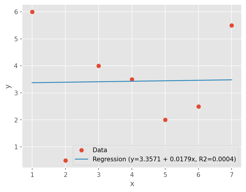
다음 분포에 대해서 추세선과 결정계수를 구하시오
\([6, 0.5, 4, 3.5, 2, 2.5, 5.5]\)
# Data
y = np.array([6, 0.5, 4, 3.5, 2, 2.5, 5.5])
n = len(y)
x = np.arange(n) + 1

# coeffcient a_1
a1 = (n*np.dot(x, y) - sum(x)*sum(y)) / (n*np.dot(x, x) - sum(x)**2)

# coefficient a_0
a0 = y.mean() - a1*x.mean()

# Calculate r^2
St = sum((y - y.mean())**2)
Sr = sum((y - a0  - a1*x)**2)

r2 = (St - Sr) /St
print("R2={:.4f}, R={:.4f}".format(r2, np.sqrt(r2)))

plt.plot(x, y, marker='o', linestyle='none')
plt.plot(x, a0 + a1*x)

plt.legend(['Data', 'Regression (y={:.4f} + {:.4f}x, R2={:.4f})'.format(a0, a1, r2)])
plt.xlabel('x')
plt.ylabel('y')
R2=0.0004, R=0.0198
Text(0, 0.5, 'y')
DIY#
행렬 크기에 따라 Gauss Elimination 계산 비용 과 상중대각행렬의 계산 비용 을 선형 회귀분석을 하시오. 이때 결정계수를 비교하시오.
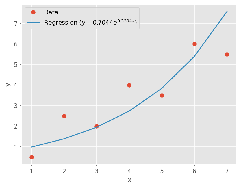
비선형 관계식의 선형화#
간단한 비선형 관계식의 경우 선형화를 통해 선형 회귀분석이 가능함.
지수모델, 멱 방정식
\[ y = \alpha_1 e^{\beta_1 x}, y = \alpha_2 x^{\beta_2 x} \]다음과 같이 변형해서 선형 회귀분석으로 \(\alpha_i, \beta_i\) 산출
\[ \log(y) = \log(\alpha_1) + \beta_1 x \]
포화 성장률 방정식
\[ y = \alpha_3 \frac{x}{\beta_3 + x} \]다음과 같이 변형
\[ \frac{1}{y} = \frac{\beta_3}{\alpha_3} \frac{1}{x} + \frac{1}{\alpha_3} \]
# 지수모델
y = np.array([0.5, 2.5, 2.0, 4.0, 3.5, 6.0, 5.5])
x = np.array(range(1, 8))

# 지수로 변환
yl = np.log(y)

# coeffcient a_1
a1 = (n*np.dot(x, yl) - sum(x)*sum(yl)) / (n*np.dot(x, x) - sum(x)**2)

# coefficient a_0
a0 = yl.mean() - a1*x.mean()

# alpha, beta
alpha, beta = np.exp(a0), a1

# regression
yst = alpha*np.exp(beta*x)

# Plot
plt.plot(x, y, marker='o', linestyle='none')
plt.plot(x, yst)

plt.legend(['Data', r'Regression ($y={:.4f}e^{{{:.4f}x}}$)'.format(alpha, beta)])
plt.xlabel('x')
plt.ylabel('y')
Text(0, 0.5, 'y')
다항식 선형 회귀분석#
다향식으로 구성한 모델: \(\tilde{y} = a_0 + a_1 x + a_2 x^2 + ... + a_n x^n\)
잔차의 제곱합 최소화:
\[ S_r = \sum (y_i - \tilde{y}(x_i))^2 \]\[ \frac{\partial S_r}{\partial a_0}=0, \frac{\partial S_r}{\partial a_1}=0, ... \frac{\partial S_r}{\partial a_n}=0, \]계수 \(a_0, a_1,...,a_n\)
\[\begin{split}\begin{bmatrix} \sum 1 & \sum x_i & \sum x_i^2 & & \sum x_i^n \\ \sum x_i & \sum x_i^2 & \sum x_i^3 & & \sum x_i^{n+1} \\ & & & & \\ \sum x_i^n & \sum x_i^{n+1} & \sum x_i^{n+3} & & \sum x_i^{2n} \end{bmatrix} \begin{bmatrix} a_0 \\ a_1 \\ \\ a_n \end{bmatrix} = \begin{bmatrix} \sum y_i \\ \sum x_i y_i \\ \\ \sum x_i^n y_i \end{bmatrix} \end{split}\]
예제#
교재 15.5 예제를 2차식으로 회귀 분석
y = np.array([2.1, 7.7, 13.6, 27.2, 40.9, 61.1])
x = np.array(range(6))

n = len(y)

A = np.array(
[[n, sum(x), sum(x**2)],
[sum(x), sum(x**2), sum(x**3)],
[sum(x**2), sum(x**3), sum(x**4)]])

b = np.array([sum(y), sum(x*y), sum(x**2*y)])

a = np.linalg.solve(A, b)
print(a)

St = sum((y - y.mean())**2)
Sr = sum((y - a[0]  - a[1]*x - a[2]*x**2)**2)

r2 = (St - Sr) /St
print(r2, np.sqrt(r2))
[2.47857143 2.35928571 1.86071429]
0.9985093572984048 0.9992544006900369
plt.plot(x, y, marker='o', linestyle='none')

xi = np.linspace(0, 5, 51)
plt.plot(xi, a[0] + a[1]*xi + a[2]*xi**2)

plt.legend([
    'Data',
    'Regression ($y={:.4f} + {:.4f}x + {:.4f}x^2$)'.format(*a),
])
plt.xlabel('x')
plt.ylabel('y')
Text(0, 0.5, 'y')

DIY#
분포를 받으면 n차 회귀분석을 할 수 있는 함수를 만드시오.
계수를 반환하시오
상관계수를 출력하시오
keyword argument
is_show가 True 일 때는 그래프를 그리시오.
다중 선형 회귀 분석#
독립 변수가 여러 개일 때도 마찬가지로 회귀분석 한다.
다중함수 모델: \(y = a_0 + a_1 x_1 + a_2 x_2\)
잔차의 제곱합 최소화:
\[ S_r = \sum (y_i - \tilde{y}(x_i))^2 \]\[ \frac{\partial S_r}{\partial a_0}=0, \frac{\partial S_r}{\partial a_1}=0, \frac{\partial S_r}{\partial a_2}=0, \]계수 \(a_0, a_1,...,a_n\)
\[\begin{split}\begin{bmatrix} n & \sum x_{1i} & \sum x_{2i} \\ \sum x_{1i} & \sum x_{1i}^2 & \sum x_{1i} x_{2i} \\ \sum x_{2i} & \sum x_{1i} x_{2i} & \sum x_{2i}^2 \end{bmatrix} \begin{bmatrix} a_0 \\ a_1 \\ a_2 \end{bmatrix} = \begin{bmatrix} \sum y_i \\ \sum x_{1i} y_i \\ \sum x_{2i} y_i \end{bmatrix} \end{split}\]
Scipy 활용#
Scipy 에는 선형 회귀분석과 비선형 회귀분석 함수를 제공한다.
선형 회귀분석:
scipy.stats.linregress함수다항함수 적합:
numpy.polyfit함수numpy.poly1d로 계산https://numpy.org/doc/stable/reference/generated/numpy.polyfit.html
비선형 회귀분석:
scipy.optimize.curve_fit함수
# 예제
y = np.array([2.1, 7.7, 13.6, 27.2, 40.9, 61.1])
x = np.array(range(6))

# Compute coefficients
z = np.polyfit(x, y, deg=2)
print(z)

# Make function using the coefficeint
approxf = np.poly1d(z)

# Plot

plt.plot(x, y, marker='o', linestyle='none')

xi = np.linspace(0, 5, 51)
plt.plot(xi, approxf(xi))

plt.legend([
    'Data',
    'Regression ($y={:.4f} + {:.4f}x + {:.4f}x^2$)'.format(*z[::-1]),
])
plt.xlabel('x')
plt.ylabel('y')
[1.86071429 2.35928571 2.47857143]
Text(0, 0.5, 'y')